XLOOKUP wildcard match example

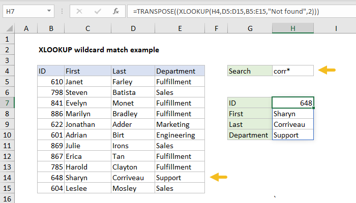
Working from the inside out, XLOOKUP is configured to find the value in H4 in the Last name column, and return all fields. In order to support wildcards, match_mode is provided as 2:

XLOOKUP(H4,D5:D15,B5:E15,2) // match Last, return all fields

• The lookup_value comes from cell H4
• The lookup_array is the range D5:D15, which contains Last names
• The return_array is B5:E15, which contains all fields
• The not_found argument is set to “Not found”
• The match_mode is 2, to allow wildcards
• The search_mode is not provided and defaults to 1 (first to last)

Since H4 contains “corr*”, XLOOKUP finds the first Last name beginning with “corr” and returns all four fields in a horizontal array:

{648,"Sharyn","Corriveau","Support"}

This result is returned directly to the TRANSPOSE function:

=TRANSPOSE({648,"Sharyn","Corriveau","Support"})

The TRANSPOSE function changes the array from horizontal to vertical:

{648;"Sharyn";"Corriveau";"Support"} // vertical array

and the array values spill into the range H7:H10.

With implicit wildcard

In the example above, the asterisk wildcard (*) is entered explicitly into the lookup value. To pass in the wildcard implicitly, you can adjust the formula like this:

=TRANSPOSE((XLOOKUP(H4&"*",D5:D15,B5:E15,"Not found",2)))

Above, we concatenate the asterisk wildcard (*) to the value in H4 in the formula itself. This will append the asterisk to any value entered in H4, and XLOOKUP will perform a wildcard lookup.

Dynamic Array Formulas are available in Office 365 only.